

Understanding Machine Learning: The Five Tribes Framework
A Comprehensive Guide to ML Approaches, Tasks, and Transparency
Machine learning isn't magic. At its core, every ML algorithm does the same thing: it takes data organized as points in space and transforms those points into decisions or predictions. Think about it in 2D or 3D—the only dimensions we can actually visualize. Each data point has a position defined by its features (age, income, blood pressure, whatever matters for your problem). The algorithm's job is to find patterns in how these points are arranged: measuring distances between them, finding directions that separate different groups, drawing boundaries that divide the space into decision regions.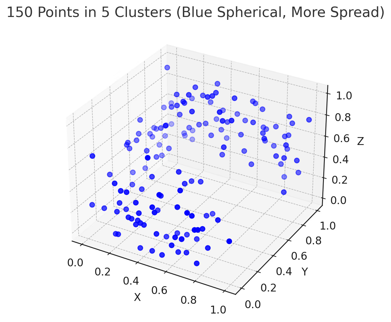
The "Five Tribes" framework, introduced by Pedro Domingos in The Master Algorithm (2015), organizes ML approaches by their fundamental philosophy about how to find these patterns. Understanding which tribe an algorithm belongs to tells you what kind of data it needs, what output it produces, and when you should use it. This isn't just academic taxonomy—it's practical decision-making for anyone building ML systems.
The Five Tribes of Machine Learning
Each tribe has a different answer to the question: "How do you transform points in space into predictions?"
1. SYMBOLISTS
Representative Algorithms: Decision Trees, Rule-Based Systems, Inductive Logic Programming
How do they learn?
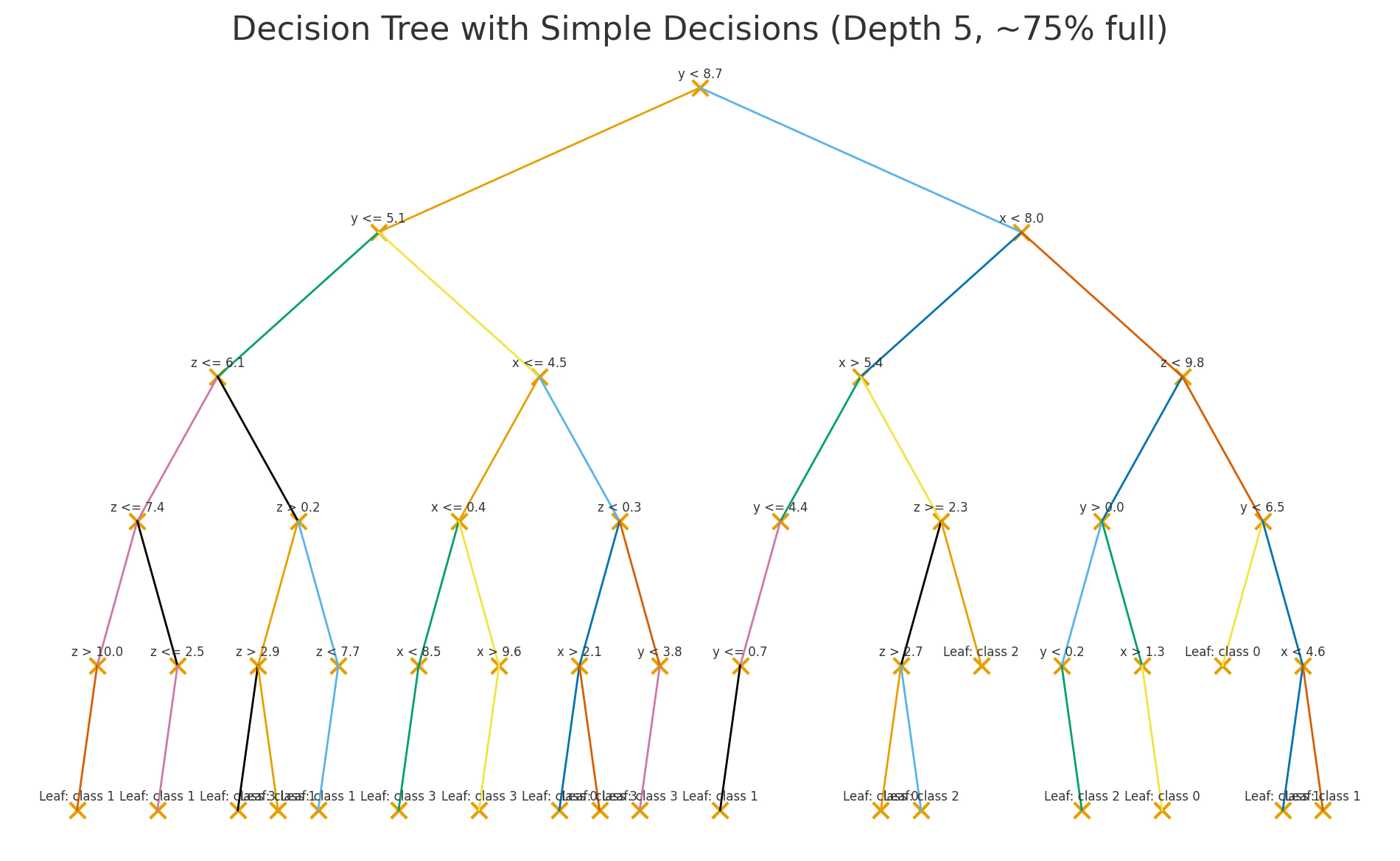
Symbolists search for logical rules by recursively partitioning the space. Imagine drawing lines (in 2D) or planes (in 3D) that separate different classes of points. Each split creates a decision: "IF feature_X > threshold THEN go left, ELSE go right." The algorithm builds a tree of these decisions until each region is pure (or close enough). This mirrors human reasoning—testing hypotheses and building explicit decision structures.
What data do they need?
Structured, tabular data with meaningful feature names. Works best with categorical or discrete variables, though continuous features are fine. Need clean, labeled data, but smaller datasets acceptable—hundreds to thousands of examples often sufficient. The key is that features must mean something interpretable: "age," "income," "blood_pressure" work; "pixel_234" doesn't.
What output do they produce and how to use it?
Explicit IF-THEN rules that humans can read:
- Decision trees as visual flowcharts
- Rule sets: "IF age > 65 AND blood_pressure > 140 THEN high_risk"
- Logic programs with clear predicates
Usage guidelines:
- Direct implementation: Rules can be coded into production systems without the model
- Human verification: Domain experts can validate each rule—critical for medical/legal applications
- Regulatory compliance: Rules provide audit trails (if a human doctor must explain "why did you diagnose this?", the same standard should apply to AI)
- Feature engineering insights: Rules reveal which feature combinations matter most
Watch out for:
- Deep trees overfit—use pruning or max_depth limits
- Hard boundaries (age > 65) may not reflect reality's continuity
- Rules inherit data biases explicitly and visibly
Transparency: 🦉🦉🦉🦉🦉 Both algorithm and output are interpretable (Huysmans et al., 2011).
2. CONNECTIONISTS
Representative Algorithms: Neural Networks, Deep Learning, Perceptrons
How do they learn?
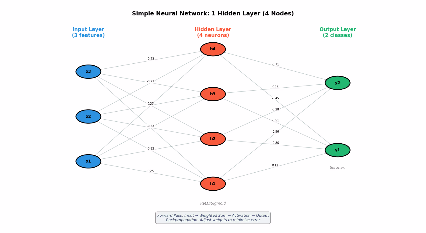
Connectionists transform the input space through layers of weighted combinations. Each neuron computes a weighted sum of its inputs, applies a non-linear activation, and passes the result forward. Learning happens via backpropagation: make a prediction, calculate error, adjust weights to reduce that error. Deep networks create increasingly abstract representations—imagine the space being stretched, rotated, and folded until different classes become separable by a simple boundary in the final layer.
What data do they need?
Massive amounts—typically thousands to millions of examples. Excel with unstructured, high-dimensional data where raw features don't mean much: image pixels, text tokens, audio waveforms. The network learns its own spatial representation. Require GPU computing for deep architectures.
What output do they produce and how to use it?
- Classification: Probability distributions over classes [0.92 cat, 0.05 dog, 0.03 rabbit]
- Regression: Continuous predictions (no inherent uncertainty)
- Embeddings: Dense vectors representing learned features
- Attention weights: For transformers, showing what the model "looked at"
Usage guidelines:
- Set probability thresholds: Don't blindly take argmax. High-stakes decisions should require 95%+ confidence; flag uncertain cases for human review
- Calibrate outputs: Raw neural network probabilities are often overconfident (Guo et al., 2017). Use temperature scaling
- Distance from decision boundary: In final layer space, points far from boundaries are more confident
- Use embeddings for similarity: Good for recommendation and retrieval, but individual dimensions aren't interpretable
Watch out for:
- Networks give confident predictions even when wrong—no "I don't know" signal
- Adversarial vulnerability: tiny input perturbations can flip predictions
- Distribution shift: performance degrades on data unlike training set, often silently
- Attention weights ≠ explanation (high attention doesn't mean causal importance)
Transparency: 🦉 Highly opaque despite mathematical precision (Lipton, 2018).
3. EVOLUTIONARIES
Representative Algorithms: Genetic Algorithms, Genetic Programming, Evolutionary Strategies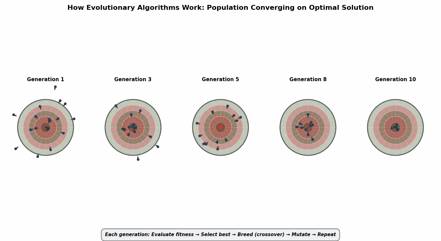
How do they learn?
Evolutionaries simulate natural selection on candidate solutions. Create a population, evaluate fitness, breed the best performers through crossover and mutation, repeat for generations. No gradients needed—pure survival of the fittest. Instead of transforming data points directly, they search the space of possible algorithms or parameter settings.
What data do they need?
Any type, but primarily used for optimization problems where gradient information isn't available. Can work with small to medium datasets. Need a clear fitness function to evaluate solution quality. Often applied to combinatorial problems or structure search (like neural architecture search) rather than direct prediction.
What output do they produce and how to use it?
- Optimized parameter sets
- Evolved program structures (genetic programming can create actual code)
- Neural network architectures
- Population of solutions (diversity, not just one answer)
Usage guidelines:
- Test top-N solutions: Use multiple from final population, not just the best
- Validate on holdout data: Evolved solutions can overfit to fitness function
- Inspect evolved programs: If genetic programming generated code, review it for correctness
- Simplify: Evolved solutions often bloated—prune unnecessary complexity
Watch out for:
- Stochastic: different runs give different answers—need multiple runs for confidence
- Computationally expensive: evolution can take hours or days
- Fitness function gaming: evolution finds unintended shortcuts if fitness poorly designed
Transparency: 🦉🦉 Algorithm process opaque (stochastic), but evolved solution can be interpretable or not (Eiben & Smith, 2015).
4. BAYESIANS
Representative Algorithms: Naive Bayes, Bayesian Networks, Gaussian Processes, Hidden Markov Models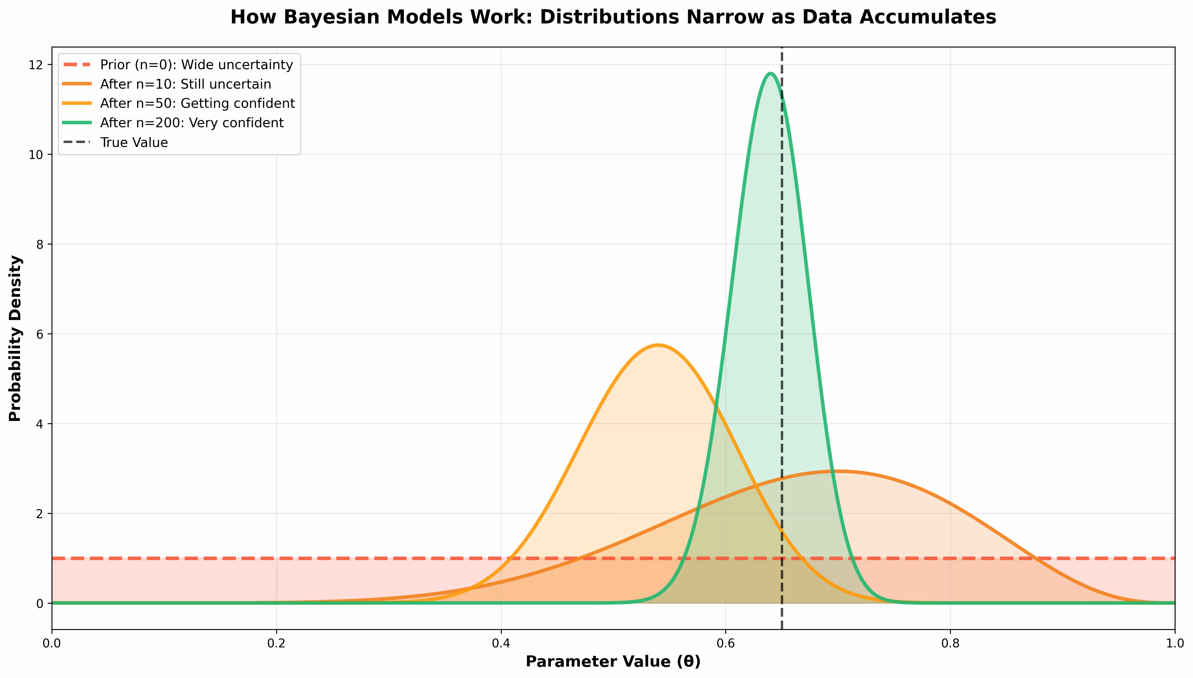
How do they learn?
Bayesians update probability distributions using Bayes' theorem: P(hypothesis|data) ∝ P(data|hypothesis) × P(hypothesis). Learning means updating beliefs about where points belong and what boundaries separate them. Instead of finding the single best boundary, Bayesians maintain distributions over all possible boundaries, weighted by their probability given the data.
What data do they need?
Can work with small datasets by incorporating prior knowledge. Handle missing data naturally through marginalization. Best with structured data where relationships between variables matter. The key advantage: you can encode expert knowledge as priors before seeing any data.
What output do they produce and how to use it?
- Probability distributions: Full distributions over predictions, not just point estimates
- Uncertainty quantification: Confidence intervals for every prediction
- Posterior probabilities: Updated beliefs P(hypothesis|data)
Usage guidelines:
- Report full distributions: "90% chance patient recovers in 5-7 days, 10% chance takes 10+ days"—don't just give the mean
- Risk assessment: Calculate P(adverse outcome) with uncertainty bounds
- Credible intervals: Report 95% credible intervals: "Effect size between 0.3 and 0.8 with 95% probability"
- Sequential decisions: Update beliefs as new data arrives (clinical trials, A/B tests)
- Communicate uncertainty: Natural for explaining confidence to stakeholders
Watch out for:
- Results depend on priors—test multiple priors to ensure robustness
- MCMC sampling can be slow for complex models
- Small data + weak priors = unreliable posteriors (garbage in, garbage out applies to priors too)
Transparency: 🦉🦉🦉🦉 Probabilistic reasoning is interpretable, though complex graphical models can become opaque (Ghahramani, 2015).
5. ANALOGIZERS
Representative Algorithms: Support Vector Machines (SVMs), k-Nearest Neighbors (k-NN), Kernel Methods, Linear/Logistic Regression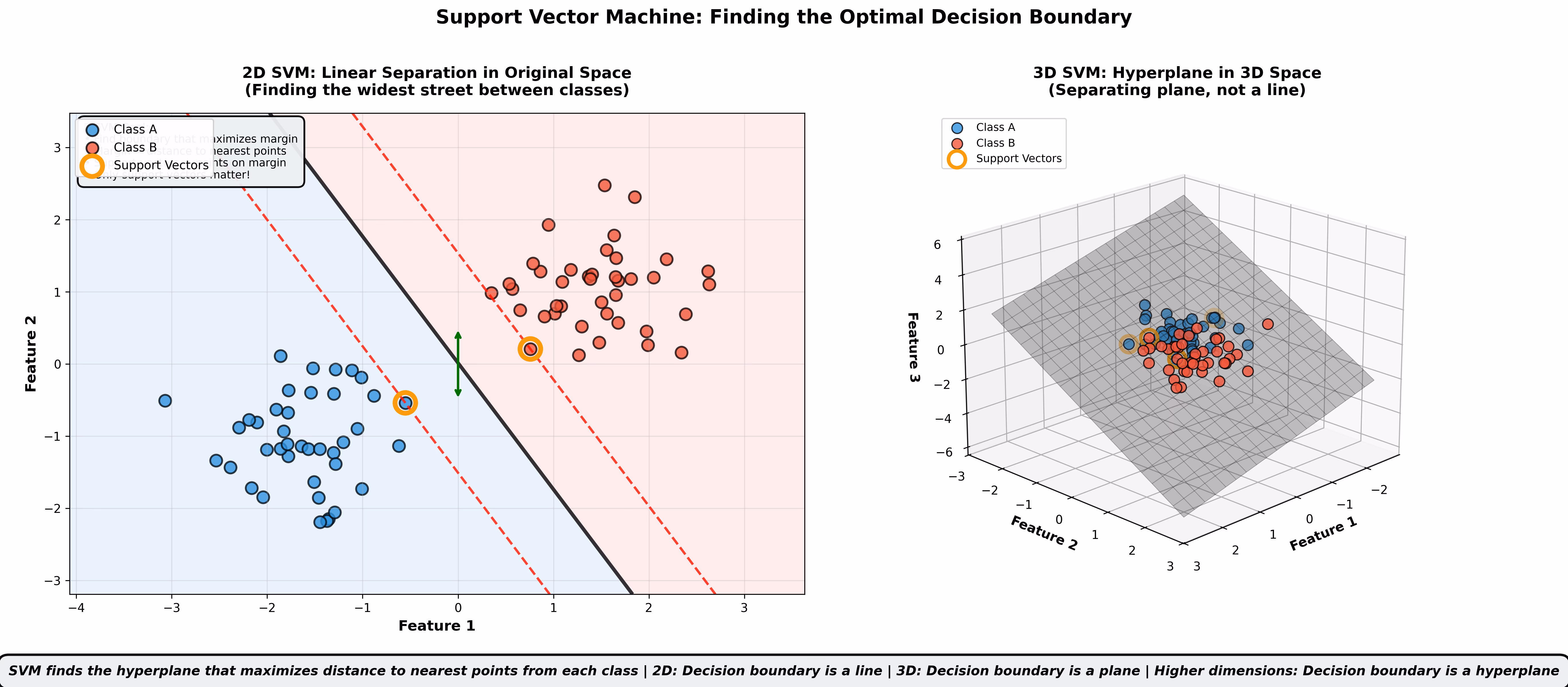
How do they learn?
Analogizers recognize patterns through similarity and distance. The core philosophy: similar points in space should have similar predictions. Linear models find hyperplanes that separate classes by maximizing margin. SVMs use kernel tricks to measure similarity in transformed spaces. k-NN simply memorizes training points and predicts based on nearest neighbors. All fundamentally about: measure distance, draw boundaries, classify by proximity.
What data do they need?
Structured, feature-based data. Linear methods need approximately linear relationships (or carefully engineered features that create linearity). Kernel methods handle non-linear relationships through space transformations. Work across small to large datasets. Critical: Feature scaling matters hugely—distance-based methods are sensitive to feature magnitudes.
What output do they produce and how to use it?
Linear Models:
- Feature coefficients showing effect direction and magnitude
- Predictions with standard errors
Usage: Coefficients are directly interpretable. Positive coefficient = feature increases prediction. "Increasing credit score by 50 points decreases default probability by 5%" is actionable. If a human banker must explain why they denied a loan, an AI using linear regression can provide the same explanation: "Income too low (coefficient: -0.3), debt-to-income too high (coefficient: +0.5)."
SVMs:
- Decision boundaries and support vectors
- Distance to boundary (confidence proxy)
Usage: Points far from decision boundary = more confident. Use decision_function() to get distance values, set acceptance thresholds (e.g., only accept if distance > 1.0). Support vectors are the "edge cases" defining the boundary—examining them reveals what's difficult to classify.
k-NN:
- Predictions based on k nearest neighbors
- The actual neighbors themselves (most interpretable!)
Usage: Explain by example: "This loan is high-risk because it resembles these 5 previous defaults." Show the actual training examples. This is the most interpretable ML method for non-technical audiences—everyone understands reasoning by analogy.
Watch out for:
Linear Models:
- Assumes linear relationships (check residual plots)
- Multicollinearity makes coefficients unstable
- Coefficients only comparable if features scaled identically
SVMs:
- Non-linear kernels (RBF) lose interpretability despite clear algorithmic optimization
- No native probability outputs—need Platt scaling
- Slow on large datasets (>100k samples)
k-NN:
- Curse of dimensionality: performance degrades with many features (>20)
- Must store entire training set (memory intensive)
- Prediction slow (searches all training points)
Transparency: 🦉🦉🦉🦉 for linear models; 🦉🦉🦉 for kernel SVMs (Cortes & Vapnik, 1995; Hastie et al., 2009).
Comparison Table
| Tribe | How They Learn | Best Data Type | Output Type | Transparency |
|---|---|---|---|---|
| Symbolists | Recursive partitioning | Structured, tabular | Explicit rules | 🦉🦉🦉🦉🦉 |
| Connectionists | Gradient descent on weights | Unstructured, massive | Probabilities, embeddings | 🦉 |
| Evolutionaries | Natural selection | Any (optimization) | Variable structures | 🦉🦉 |
| Bayesians | Probabilistic updating | Structured, any size | Distributions + uncertainty | 🦉🦉🦉🦉 |
| Analogizers | Similarity/distance | Structured, features | Boundaries, coefficients | 🦉🦉🦉-🦉🦉🦉🦉 |
The Five Machine Learning Tasks
Tribes are approaches—how you solve problems. Tasks are what you're solving. Here are the five core ML tasks:
1. Classification: Assigning items to discrete categories (spam/not spam, disease present/absent, cat/dog/rabbit)
2. Regression: Predicting continuous numbers (house prices, temperature, stock returns)
3. Clustering: Grouping similar items without predefined labels (customer segmentation, document organization)
4. Recommendation: Suggesting items users might like (Netflix shows, Amazon products, job matches)
5. Prediction: Forecasting future sequences or events (stock prices over time, next word in a sentence, weather)
Key insight: Clustering isn't a tribe—it's a task that appears across multiple tribes. k-means clustering is Analogizers (distance-based). Hierarchical clustering is Symbolists (tree structures). Gaussian Mixture Models are Bayesians (probabilistic). Same task, different tribal approaches.
Regression lives primarily in Analogizers (linear regression is the foundation) but appears across tribes: decision trees do regression, neural networks do regression, Gaussian processes (Bayesian) do regression.
Tribes × Tasks Performance Matrix
No single tribe dominates all tasks—this is the "No Free Lunch" theorem (Wolpert & Macready, 1997). The best algorithm depends on your data structure and problem type.
| Tribe | Classification | Regression | Clustering | Recommendation | Prediction |
|---|---|---|---|---|---|
| Symbolists | 🫖🫖🫖🫖🫖 | 🦉🦉🦉🦉 | 🫖🫖🫖 | 🦉🦉🦉 | 🫖🫖🫖 |
| Analogizers | 🫖🫖🫖🫖🫖 | 🦉🦉🦉🦉🦉 | 🫖🫖🫖🫖 | 🦉🦉🦉🦉 | 🫖🫖🫖 |
| Bayesians | 🫖🫖🫖🫖 | 🦉🦉🦉🦉 | 🫖🫖🫖🫖 | 🦉🦉🦉 | 🫖🫖🫖🫖 |
| Evolutionaries | 🫖🫖🫖 | 🦉🦉🦉 | 🫖🫖 | 🦉🦉🦉 | 🫖🫖🫖 |
| Connectionists | 🫖🫖🫖🫖🫖 | 🦉🦉🦉🦉 | 🫖🫖🫖 | 🦉🦉🦉🦉🦉 | 🫖🫖🫖🫖🫖 |
Key patterns:
- Analogizers most versatile: Strong across all tasks, especially regression (linear regression is the gold standard)
- Connectionists dominate modern complex tasks: State-of-art for images (He et al., 2016), text (Vaswani et al., 2017), recommendations (Covington et al., 2016), and sequences
- Symbolists win interpretability: Best when decisions must be explained
- Bayesians unique for uncertainty: Only tribe that naturally quantifies "I don't know"
- Evolutionaries niche: Useful when gradients unavailable or searching for novel structures
Empirical evidence: Fernández-Delgado et al. (2014) tested 179 classifiers across 121 datasets. Random forests (Symbolist ensembles) and SVMs (Analogizers) often performed best, but simpler methods competitive on many datasets—especially with good feature engineering.
Choosing Your Tribe
| Your Situation | Recommended Tribe | Why |
|---|---|---|
| Structured data, must explain decisions | Symbolists or Analogizers (linear) | Regulatory compliance, stakeholder trust |
| Small dataset, uncertainty matters | Bayesians | Confidence intervals, works with limited data |
| Images, text, audio | Connectionists | State-of-art for unstructured data |
| Need feature importance | Analogizers (linear models) | Coefficients directly interpretable |
| Optimization without gradients | Evolutionaries | When gradient-based methods fail |
| Explain by example | Analogizers (k-NN) | Most intuitive for non-technical audiences |
The bottom line: Start by asking what kind of data you have (structured vs unstructured) and whether you must explain individual decisions. Structured data + explainability requirement = start with interpretable tribes (Symbolists, Bayesians, Analogizers). Only move to opaque models if interpretable ones genuinely underperform.
But what about the famous performance-interpretability tradeoff? Don't you have to sacrifice accuracy for interpretability? That's the biggest myth in machine learning—and it's the topic of our next post.
References
Core Framework
- Domingos, P. (2015). The Master Algorithm: How the Quest for the Ultimate Learning Machine Will Remake Our World. Basic Books.
Interpretability & Transparency
Adadi, A., & Berrada, M. (2018). "Peeking Inside the Black-Box: A Survey on Explainable Artificial Intelligence (XAI)." IEEE Access, 6, 52138-52160.
Doshi-Velez, F., & Kim, B. (2017). "Towards a rigorous science of interpretable machine learning." arXiv preprint arXiv:1702.08608.
Huysmans, J., Dejaeger, K., Mues, C., Vanthienen, J., & Baesens, B. (2011). "An empirical evaluation of the comprehensibility of decision table, tree and rule based predictive models." Decision Support Systems, 51(1), 141-154.
Liao, Q. V., & Varshney, K. R. (2022). "Human-Centered Explainable AI (XAI): From Algorithms to User Experiences." arXiv preprint arXiv:2110.10790.
Lipton, Z. C. (2018). "The mythos of model interpretability." Queue, 16(3), 31-57.
Rudin, C. (2019). "Stop explaining black box machine learning models for high stakes decisions and use interpretable models instead." Nature Machine Intelligence, 1(5), 206-215.
ML Fundamentals & Textbooks
Breiman, L. (2001). "Statistical Modeling: The Two Cultures." Statistical Science, 16(3), 199-231.
Hastie, T., Tibshirani, R., & Friedman, J. (2009). The Elements of Statistical Learning: Data Mining, Inference, and Prediction (2nd ed.). Springer.
Mitchell, T. M. (1997). Machine Learning. McGraw-Hill.
Murphy, K. P. (2012). Machine Learning: A Probabilistic Perspective. MIT Press.
Specific Algorithms
Cortes, C., & Vapnik, V. (1995). "Support-vector networks." Machine Learning, 20(3), 273-297.
Eiben, A. E., & Smith, J. E. (2015). Introduction to Evolutionary Computing (2nd ed.). Springer.
Ghahramani, Z. (2015). "Probabilistic machine learning and artificial intelligence." Nature, 521(7553), 452-459.
Goodfellow, I., Bengio, Y., & Courville, A. (2016). Deep Learning. MIT Press.
Guo, C., Pleiss, G., Sun, Y., & Weinberger, K. Q. (2017). "On calibration of modern neural networks." ICML, 1321-1330.
Performance Comparisons
Fernández-Delgado, M., Cernadas, E., Barro, S., & Amorim, D. (2014). "Do we need hundreds of classifiers to solve real world classification problems?" Journal of Machine Learning Research, 15(1), 3133-3181.
Wolpert, D. H., & Macready, W. G. (1997). "No free lunch theorems for optimization." IEEE Transactions on Evolutionary Computation, 1(1), 67-82.
Modern Deep Learning Applications
Covington, P., Adams, J., & Sargin, E. (2016). "Deep neural networks for YouTube recommendations." RecSys, 191-198.
He, K., Zhang, X., Ren, S., & Sun, J. (2016). "Deep residual learning for image recognition." CVPR, 770-778.
Vaswani, A., et al. (2017). "Attention is all you need." NeurIPS, 5998-6008.
