

At Analystrix, we pursue the work to best explain how models make decisions because transparency is key to benefitting from AI. While we do our work in XAI, we focus on nine specific questions that look into the interpretability of all AI models. We will be going through each of these questions using an example of a binary classifier.
The Framework: Nine Questions for XAI
This framework is based on the research by Liao, Q. V., & Varshney, K. R. (2021), "Human-Centered Explainable AI (XAI): From Algorithms to User Experiences," arXiv preprint arXiv:2110.10790. Their work identified these fundamental questions that users need answered to understand and trust AI systems.
The nine questions provide a comprehensive lens for evaluating AI explainability:
- Data - What data was used?
- Performance - How well does it work?
- Why - Why this prediction?
- Why Not - Why not a different prediction?
- How To Be That - What changes would alter the prediction?
- How To Still Be - How stable is this prediction?
- What If - How do changes affect outcomes?
- How - How does the system work overall?
- Output - How should outputs be used?
Let's explore each question with practical examples using a binary classifier.
1. Data
All AI models rely on data as their source of learning. Without data, AI models cannot learn the structures or pathways needed to approach solutions to problems.
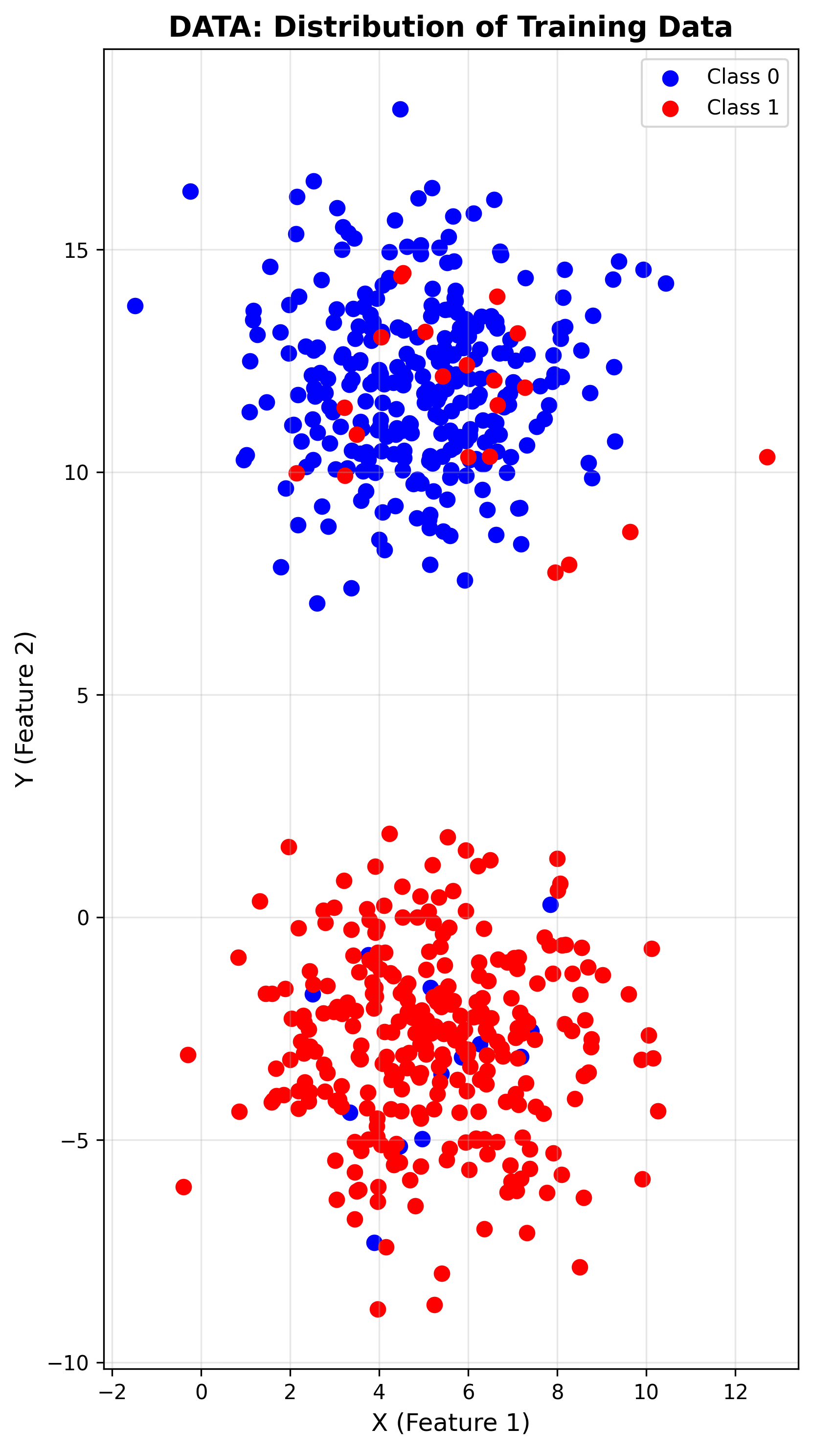
In the figure above we can see a 2D plot of the data we will be working with. You can see we have 2 classes marked in blue and red. We can also see that we do not have perfect separation of the two classes. We have some red in the blue cluster and some blue in the red cluster. Our data consists of an equal number of points for both classes (300 for each, total of 600 points).
When we look at data we are concerned with the distribution of the different classes, checking for any imbalances that will create a bias. We consider the number of features in total when categorizing a class. We would also look into issues if data has missing values, or values that are outliers. For this dataset, we have a balanced split and relatively clean data, but you can already see the challenge—the classes overlap in the feature space, which means perfect classification is impossible.
Common technique: Data profiling and bias detection methods examine source, provenance, type, size, and coverage of populations to identify potential biases before training begins.
2. Performance
This question is part of most press releases from AI companies. This focuses on the overall accuracy of the model—how often does the model produce the correct answer versus getting it wrong?
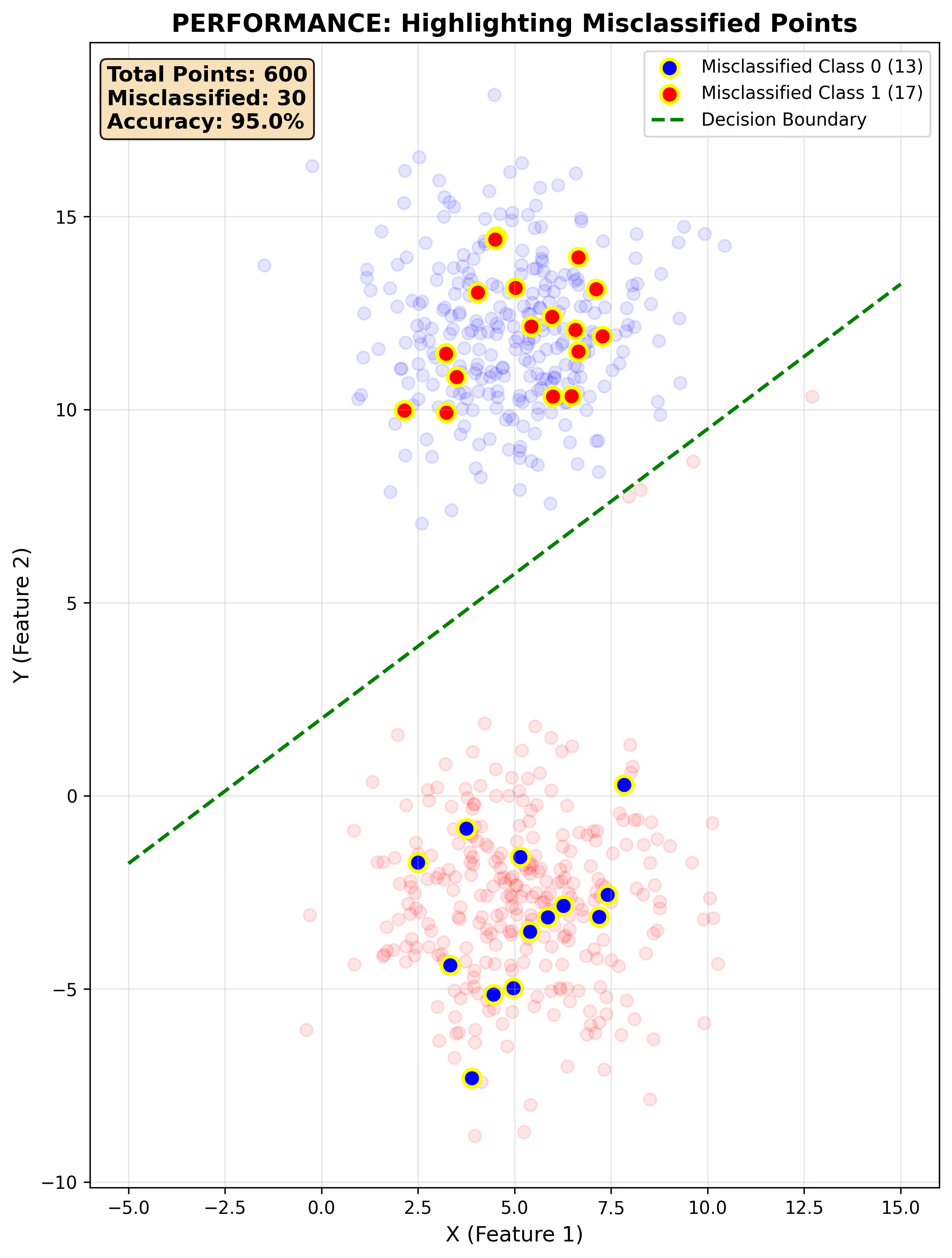
In the figure you can see that we are looking closely at the errors of our classifier which measures at about 5%, or 95% accuracy. While this is an important measurement, it can be misleading because we are only looking at the end result. We are not verifying if the model's abilities are generalized or if the model is relying on good heuristics. This can be a problem because the model might have found a reasoning path that does not align with human values. For example, a model could achieve 95% accuracy by exploiting spurious correlations or by performing well on the majority class while failing on important edge cases.
Common techniques: Beyond accuracy, we use precision, recall, F1 score, and AUC to understand model performance. For individual predictions, uncertainty estimation methods communicate confidence levels to help users understand when to trust the model.
3. Why
When looking at why, we are asking why did the model return a specific answer. This is where we start to look at feature importance and bias detection.
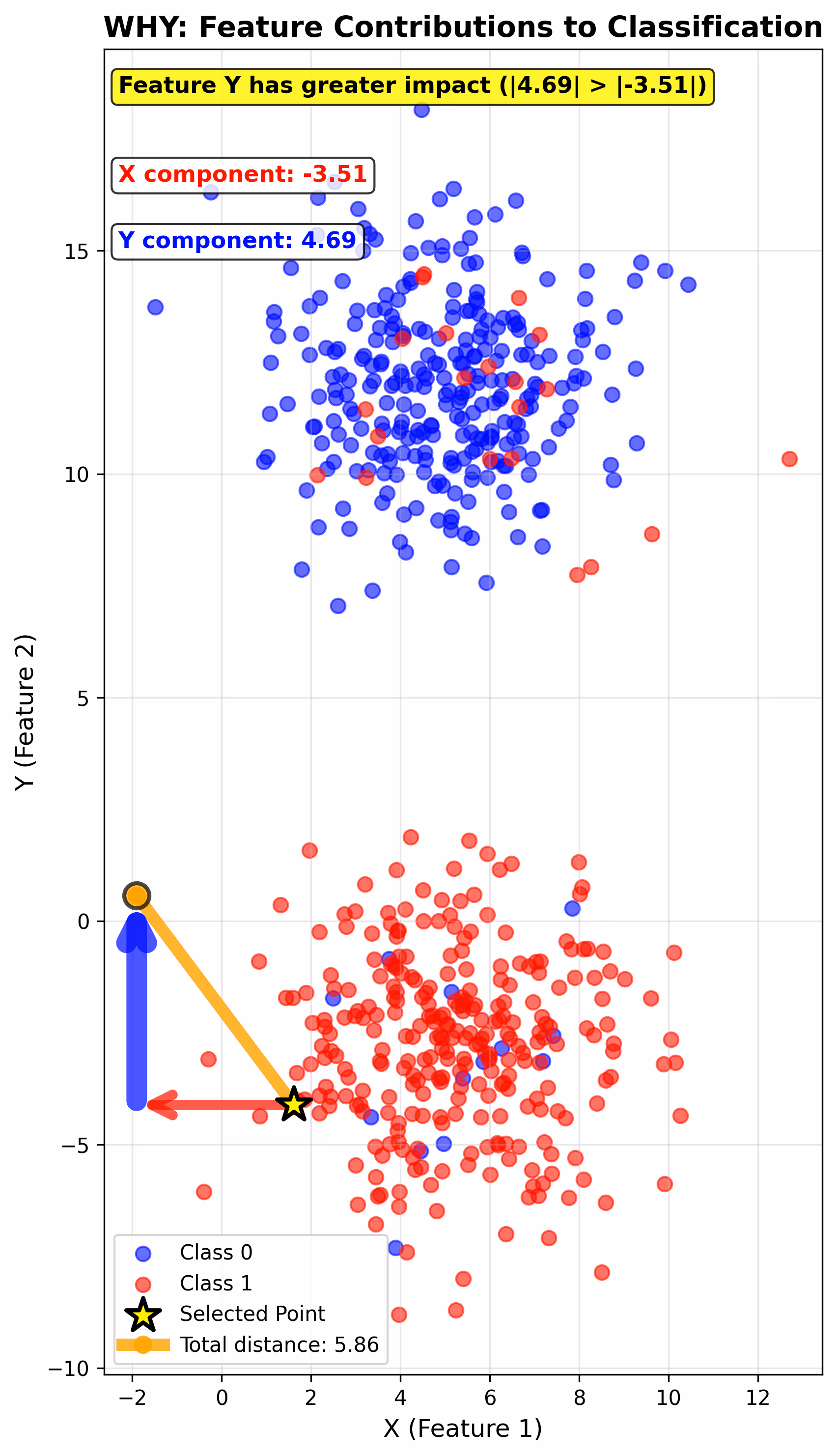
In the figure you can see that we selected a point and we are measuring the distance to the decision boundary. We then decompose the distance vector into its components. The component with the larger magnitude or value contributes more to the given classification. In this example, Feature Y (the vertical component) has a magnitude of 4.69 while Feature X has -3.51, so Feature Y is the primary driver for why this point is classified as it is. This gives us a local explanation—understanding what matters for this specific prediction.
Common techniques: LIME (Local Interpretable Model-Agnostic Explanations) and SHAP (Shapley Additive Explanations) are the most popular methods for answering "why" questions. LIME creates a simple linear model around the prediction to approximate feature importance, while SHAP uses game theory to assign credit to each feature.
4. Why Not
Here we are interested in understanding why the model did not answer a specific way for an input feature. This is about diagnosis—what is it about this input that keeps it from being classified as the target class?

In the figure we see a point selected and a line drawn showing the separation distance to the decision boundary. This represents the total gap keeping the point from crossing over from the predicted class to the target class. In this case, the point is currently Class 0 (blue), and the separation distance of 4.16 units represents what fundamentally differentiates it from Class 1. This is different from the next question because here we're focused on understanding the separation, not on how to change it.
Common techniques: Contrastive Explanation Method (CEM) and counterfactual generation algorithms identify what features determine the current prediction and what changes would lead to the alternative outcome. These methods can also use example-based approaches like ProtoDash to show prototypical examples from the other class.
5. How To Be That
This is where we look into another theme of XAI: counterfactuals. The goal in this approach is to determine how much input features need to change to get a specific answer from the model.
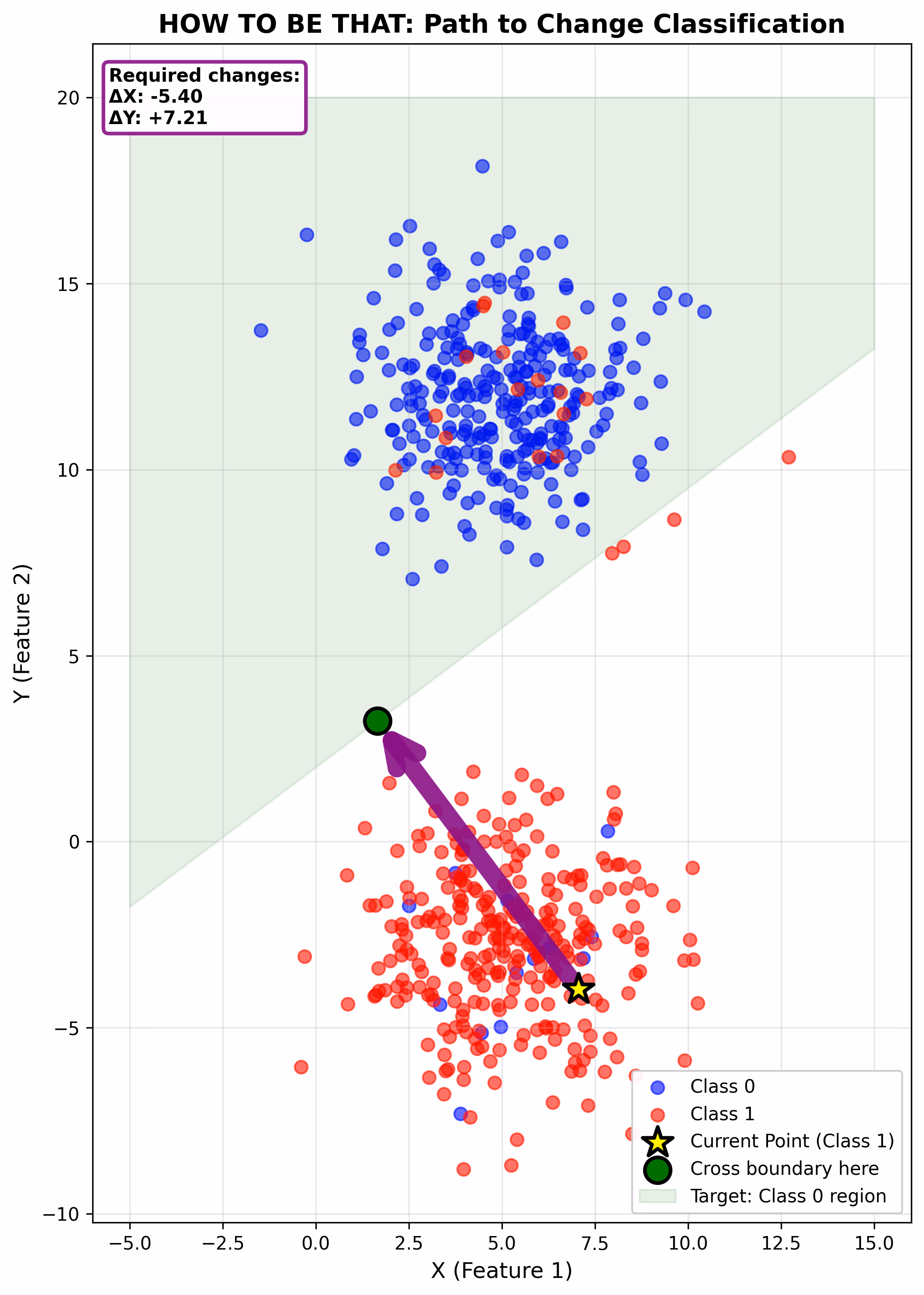
The figure shows a point being selected and an arrow being drawn to the decision boundary. This line shows the minimum changes to input data to get a new classification from the model. The required changes are ΔX: -5.40 and ΔY: +7.21, for a total path of 9.01 units. This is similar to Why Not in appearance, but the difference is in the objective of the approaches. Why Not is about understanding what about an input makes it different from the target class. How To Be That is about determining the specific, actionable changes needed to cross the boundary—making this prescriptive rather than diagnostic.
Common techniques: DiCE (Diverse Counterfactual Explanations) and counterfactual generation algorithms identify minimum changes needed to alter predictions. These methods focus on finding actionable recourse—changes that are realistic and achievable for the user to implement.
6. How To Still Be
We want to determine how sensitive a model answer is for a specific input. This involves developing methods to generate perturbations or small changes to the input features to explore around the input space.
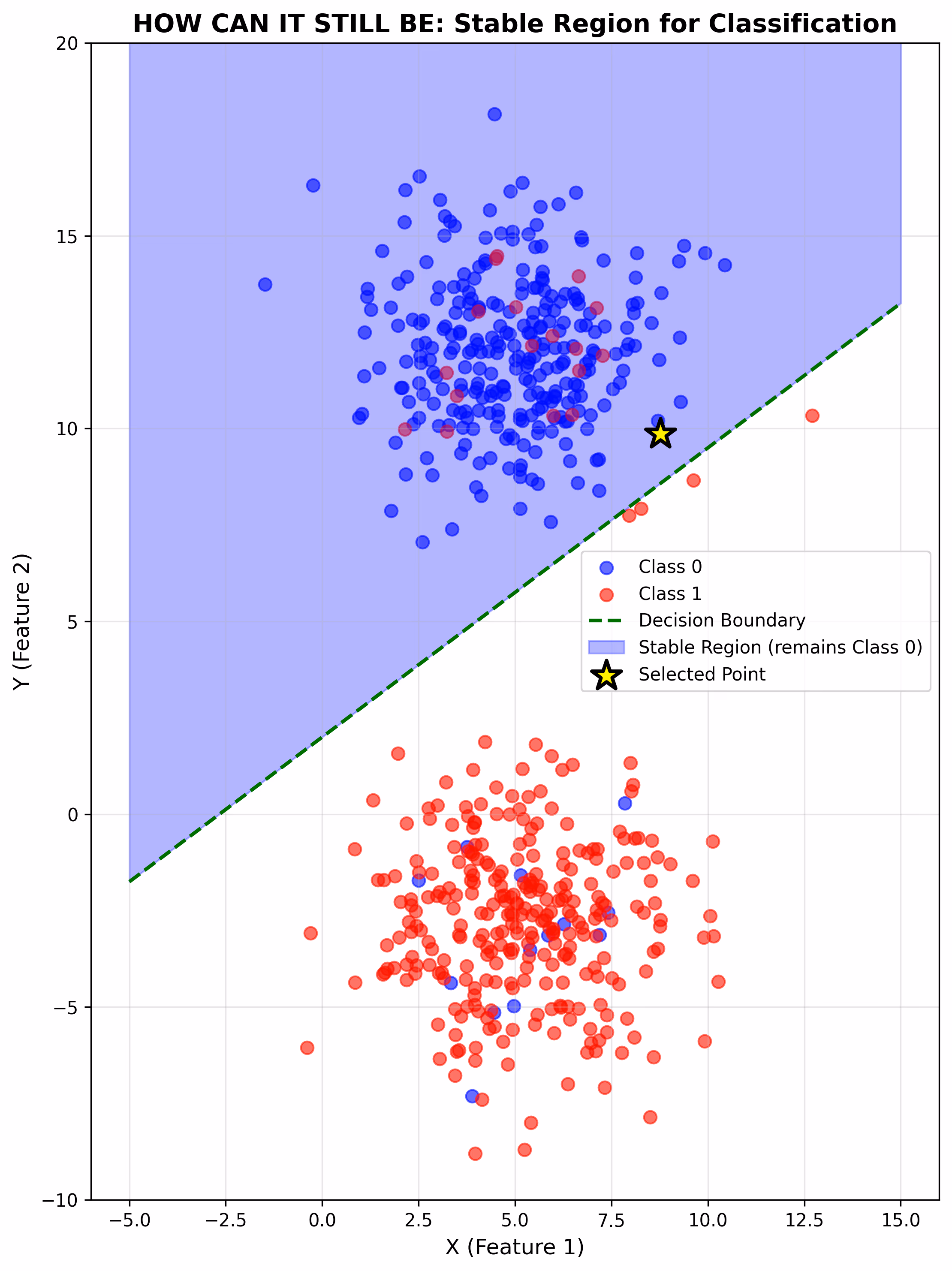
In this figure we can see that we have identified a region that represents the space of the predicted classification. Everything within this blue shaded region will be classified as Class 0. This tells us about stability—how much can we wiggle the input features before the classification changes? A larger stable region means the prediction is more robust to small variations in the input. A point near the boundary has low stability, while a point deep in the region has high stability.
Common techniques: Anchors generate rules that guarantee the same prediction within a defined region, while CEM can identify feature ranges that preserve the classification. These methods help understand prediction stability and robustness to small input changes.
7. What If
We add an input that is not part of the training data and evaluate how the model classifies the point. But more importantly, we can systematically explore how predictions change as we vary features.

The figure shows a test point at (7.66, -1.82) classified as Class 1. The vertical dashed line demonstrates systematic exploration—what if we keep X constant at 7.66 but vary Y? The orange circles mark where the prediction flips from one class to another. Below Y ≈ 7.7, the model predicts Class 1. Above that threshold, it predicts Class 0. This systematic exploration is what makes "what if" analysis powerful—we're not just testing one point, we're understanding how the model behaves across a range of inputs.
This question is about generalization and sensitivity. We want to see how the model handles new, unseen data and how sensitive predictions are to changes in specific features. This is critical for deployment because in the real world, you're always dealing with what-if scenarios.
Common techniques: Partial Dependence Plots (PDP), Accumulated Local Effects (ALE), and Individual Conditional Expectation (ICE) plots systematically explore how predictions change when features are modified. These techniques generate curves showing the relationship between input changes and model outputs across the full range of feature values, similar to our vertical exploration line but extended across the entire feature space.
8. How
This is the biggest question in XAI. The goal is to provide a global explanation for how the model answers based on the input. Ideally we want the explanation to be discrete, orderly, and understandable.
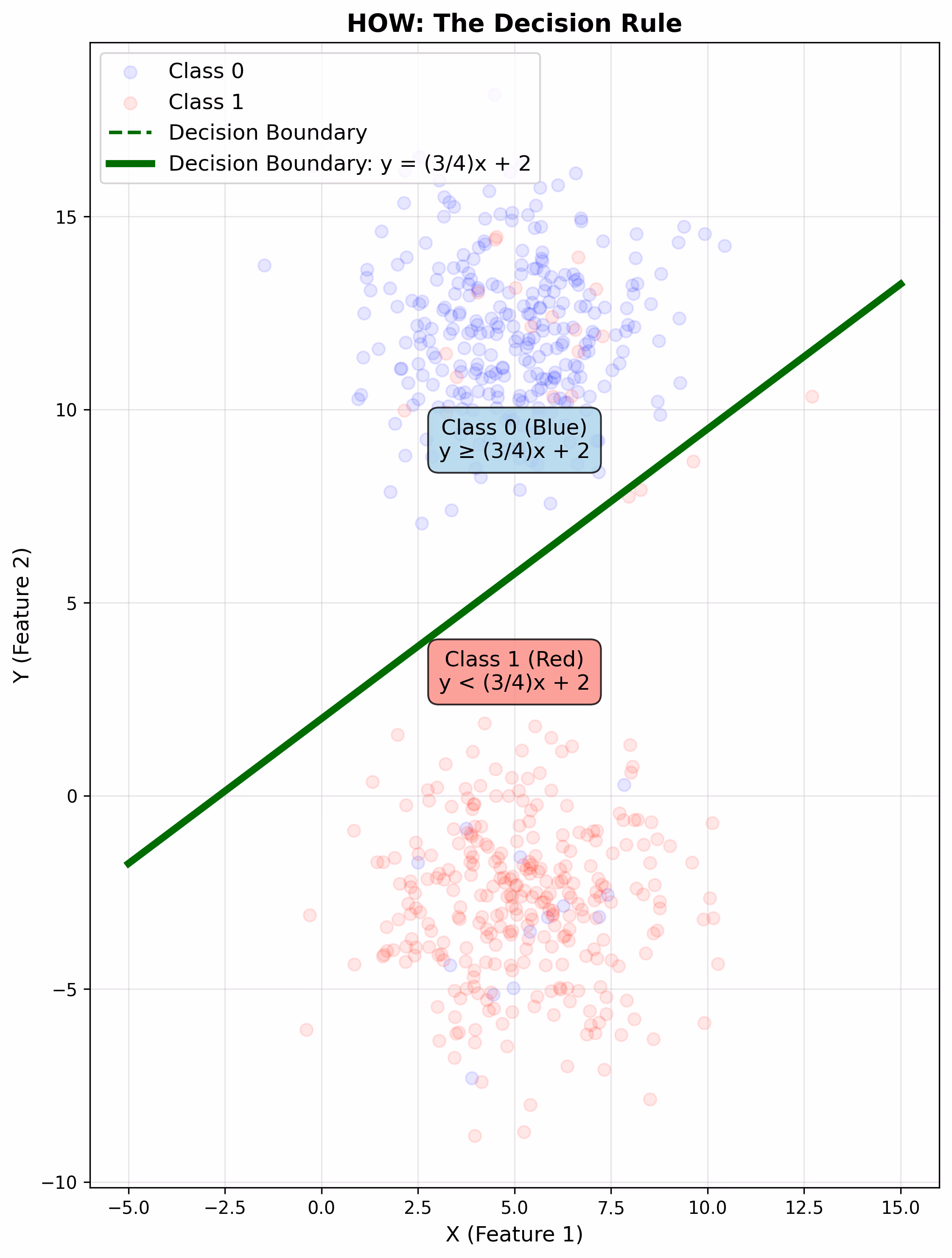
In this figure, the defined decision boundary is the How. It is a bright line that cuts across the two classes, with one class on one side and the other class on the other. The decision rule is y = (3/4)x + 2, which means the model uses a simple linear relationship between the two features. Any point above this line is Class 0, any point below is Class 1. This is the global explanation—the fundamental logic the model uses for all predictions. In more complex models (neural networks, ensemble methods), answering "How" becomes significantly harder because the decision boundary is not a simple line but a complex, high-dimensional surface. That's why this is the central challenge of XAI.
Common techniques: Global feature importance methods, Partial Dependence Plots (PDP), and tree surrogates approximate the overall model logic. For simpler models, the actual model weights or decision rules can serve as direct global explanations.
9. Output
This question deals with what happens with the model responses after training. We want to describe what the output of the model is, and how the output will be used.
Model Card: Mock Binary Classification Model
- Decision Boundary: Simple linear boundary (y = (3/4)x + 2)
- Output: Binary classification (0 or 1) representing two distinct classes
- Use Case: These outputs are used to provide visualizations to explain how to think about the 9 questions of XAI
- Deployment Considerations: In a real-world scenario, you would document how these classifications are used downstream—do they trigger automated actions? Are they reviewed by humans? What are the consequences of false positives versus false negatives?
Understanding the output means understanding the impact. A loan approval model and a spam filter both output binary classifications, but the stakes and requirements are completely different.
Common techniques: Model Cards and FactSheets provide comprehensive documentation about model scope, intended use, performance characteristics, ethical considerations, and limitations. These structured formats help stakeholders understand how model outputs should be interpreted and used.
Wrapping Up
I am aware that these examples are very simplified compared to more advanced models that are being used today (ChatGPT, Midjourney, etc.). The decision boundary here is a clean line, the features are two-dimensional, and the logic is transparent. Real models have thousands or millions of features, non-linear decision boundaries, and opaque internal representations.
But hopefully with these examples you will be able to think more clearly about how to address these 9 questions when evaluating the interpretability of your own models. Whether you're working with a simple logistic regression or a massive transformer, these questions still apply—they just get harder to answer as complexity increases.
When approaching model interpretability, start with the foundation. Questions 1 (Data) and 9 (Output) set the context—what went in and what comes out. Question 2 (Performance) tells you if the model works at all. From there, you can explore the local explanations (Questions 3, 4, 5, 6, 7) to understand specific predictions and edge cases. Finally, Question 8 (How) ties everything together by revealing the global decision-making logic.
This progression mirrors how you'd actually investigate a model in practice: understand the basics, examine specific cases, then synthesize a complete picture of how the system operates. In future posts, we'll explore how these questions translate to deep learning models where the answers are not nearly as neat.
References
Liao, Q. V., & Varshney, K. R. (2021). Human-Centered Explainable AI (XAI): From Algorithms to User Experiences. arXiv preprint arXiv:2110.10790. https://arxiv.org/abs/2110.10790
